前段时间在B站上发现一个宝藏课程《[让Nanite烂大街计划]手搓Nanite》, 怒斥138巨资学习一波. 学罢, 诚如课程老师在课程开始所预料的, 自己确实对Nanite这门目前游戏行业的顶尖技术袪魅不少. 有部分原因是因为课程中并未深入研究Nanite Mesh Build算法, 更多地是偏向于工程架构上的剖解. 虽觉可惜, 但也受益良多, 特以本文记录该课程中提及的关于原装虚幻Nanite与课程的实现细节.
参考材料
1. [让Nanite烂大街计划]手搓Nanite
2. Nanite源码笔记(2)-Encode(2)-batch&分页
3. 【Unity Graphics】莫顿码(Morton Code)
4. 游戏引擎随笔 0x20:UE5 Nanite 源码解析之渲染篇:BVH 与 Cluster 的 Culling
5. 为什么大多数透视投影矩阵只用垂直或水平角度来处理 FOV(视场角)?
6. 彻底理解投影矩阵(一)
7. 水平FOV与垂直FOV转换公式 以C++实现为例
8. CSE272高级渲染课程 (26) Nanite实时渲染
1. 原装虚幻Nanite核心LOD内存格式解析
FPackedHierarchyNode为Nanite核心LOD的核心数据结构之一, 其结构如下所示,
#define NANITE_MAX_BVH_NODE_FANOUT_BITS						2
#define NANITE_MAX_BVH_NODE_FANOUT						(1 << NANITE_MAX_BVH_NODE_FANOUT_BITS)

struct FPackedHierarchyNode
{
	FVector4f		LODBounds[NANITE_MAX_BVH_NODE_FANOUT];

	struct
	{
		FVector3f	BoxBoundsCenter;
		uint32		MinLODError_MaxParentLODError;
	} Misc0[NANITE_MAX_BVH_NODE_FANOUT];

	struct
	{
		FVector3f	BoxBoundsExtent;
		uint32		ChildStartReference;
	} Misc1[NANITE_MAX_BVH_NODE_FANOUT];

	struct
	{
		uint32		ResourcePageIndex_NumPages_GroupPartSize;
	#if NANITE_ASSEMBLY_DATA
		uint32 		AssemblyPartIndex;
	#endif
	} Misc2[NANITE_MAX_BVH_NODE_FANOUT];
};
上述结构为一个四叉树节点结构, 是Nanite实现的基础, 每个节点在GPU中以特定格式FPackedHierarchyNode存储.
1.1 节点存储布局
四叉树节点在GPU中通常采用连续内存布局, 每个节点占用固定字节数(208 = 52 $\times$ sizeof(uint)字节). 这种布局方式使得GPU能够高效地访问和处理节点数据. 节点结构包含以下关键部分:
$\\$ $\cdot$ LODBounds, 类型为FVector4f的数组, 大小为64字节, 其存储节点的边界信息, 用于视锥体裁剪和遮挡剔除;
$\\$ $\cdot$ ChildStartReference, 类型为uint32的数组, 长度为4, 大小为16字节, 其为四个子节点的起始索引, 指向子节点在Buffer中的位置; 通过NaniteRayTrace.ush中对于ChildStartReference的位运算可知, 其低24位为PageIndex, 高8位为ClusterIndex(注意, 一般GPU上使用小端编码).
#define NANITE_STREAMING_PAGE_GPU_SIZE_BITS				17
#define NANITE_CLUSTER_MIN_EXPECTED_GPU_SIZE_BITS			9	// Used to determine how many bits to allocate for page cluster count.
// Individual clusters can be smaller.
#define NANITE_STREAMING_PAGE_MAX_CLUSTERS_BITS				(NANITE_STREAMING_PAGE_GPU_SIZE_BITS - NANITE_CLUSTER_MIN_EXPECTED_GPU_SIZE_BITS)

#define NANITE_ROOT_PAGE_GPU_SIZE_BITS					15
#define NANITE_ROOT_PAGE_MAX_CLUSTERS_BITS				(NANITE_ROOT_PAGE_GPU_SIZE_BITS - NANITE_CLUSTER_MIN_EXPECTED_GPU_SIZE_BITS)

#define NANITE_MAX_CLUSTERS_PER_PAGE_BITS				(NANITE_STREAMING_PAGE_MAX_CLUSTERS_BITS > NANITE_ROOT_PAGE_MAX_CLUSTERS_BITS ? NANITE_STREAMING_PAGE_MAX_CLUSTERS_BITS : NANITE_ROOT_PAGE_MAX_CLUSTERS_BITS)
#define NANITE_MAX_CLUSTERS_PER_PAGE_MASK				((1 << NANITE_MAX_CLUSTERS_PER_PAGE_BITS) - 1)

const uint PageIndex = HierarchyNodeSlice.ChildStartReference >> NANITE_MAX_CLUSTERS_PER_PAGE_BITS;
const uint BaseClusterIndex = HierarchyNodeSlice.ChildStartReference & NANITE_MAX_CLUSTERS_PER_PAGE_MASK;
$\\$ $\cdot$ BoxBoundsCenter, 类型为FVector3f的数组, 长度为4, 大小为12字节, 其为LOD Bound的中心点位置;
$\\$ $\cdot$ BoxBoundsExtent, 类型为FVector3f的数组, 长度为4, 大小为12字节, 其为LOD Bound的边界范围;
$\\$ $\cdot$ MinLODError_MaxParentLODError, 类型为uint32的数组, 长度为4, 大小为16字节, 其存储节点的误差值, 用于LOD判断;
$\\$ $\cdot$ ResourcePageIndex_NumPages_GroupPartSize, 类型为uint32的数组, 长度为4, 大小为16字节, 通过NaniteEncode.cpp中使用位运算为ResourcePageIndex_NumPages_GroupPartSize赋值的逻辑可知, 其前14位为PageIndexStart, 中间9位为PageIndexNum, 末9位为GroupPartSize.
#define NANITE_MAX_CLUSTERS_PER_GROUP_BITS					9
#define NANITE_MAX_GROUP_PARTS_BITS						5

ResourcePageIndex_NumPages_GroupPartSize = (PageIndexStart << (NANITE_MAX_CLUSTERS_PER_GROUP_BITS + NANITE_MAX_GROUP_PARTS_BITS)) | (PageIndexNum << NANITE_MAX_CLUSTERS_PER_GROUP_BITS) | GroupPartSize;
$\\$ $\cdot$ AssemblyPartIndex, 目前宏NANITE_ASSEMBLY_DATA是处于关闭状态的, 且虚幻引擎在NaniteResource.h中已通过static_assert对FPackedHierarchyNode的数据结构大小作出限制(即不允许修改变量数量), 故该变量亦未被使用.
#define NANITE_ASSEMBLY_DATA						0

#if NANITE_ASSEMBLY_DATA
	#define NANITE_HIERARCHY_NODE_SLICE_SIZE_DWORDS			56
#else
	#define NANITE_HIERARCHY_NODE_SLICE_SIZE_DWORDS			52
#endif

// These are expected to match up
static_assert(NANITE_HIERARCHY_NODE_SLICE_SIZE_DWORDS == sizeof(FPackedHierarchyNode) / 4);
其逻辑结构如下图所示.

1.2 数据分块方式
Nanite将模型数据拆分为Clusters, 每个Cluster包含约128个三角形. 这种分块方式使得数据可以按需加载, 只渲染肉眼可见且有意义的细节. 剔除时可将屏幕分成若干个$8 \times 8$的屏幕块进行分块剔除.
1.3 访问模式
在GPU中访问四叉树节点时, 通常采用以下方式:
$\\$ $\cdot$ 通过节点索引定位到内存中的起始位置.
$\\$ $\cdot$ 根据节点大小(208字节) 计算子节点的偏移量.
$\\$ $\cdot$ 解码节点中的子节点索引, 获取子节点数据.
2. 逆向分析虚幻5.5.4的Nanite Mesh数据
2.1 Clusters生成过程
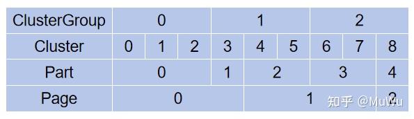
Nanite将模型分割为Clusters, 并进一步合并为Groups. 例如, 一个20号节点的四个字节点分别输出了8, 4, 2, 1个Clusters, 总共有15个Clusters, 这些Clusters被分配到内存分页的第0页上.
$\\$ Cluster Groups会进行排序, 先根据Mipmap Level进行排序, 再根据莫顿码进行排序, 这样保证同一Mipmap Level且位置相近的Group能够放到一起. 有关莫顿码可以参考【Unity Graphics】莫顿码(Morton Code). 大致就是空间中相近的点的莫顿码相近, 使用莫顿码排序可以使得空间坐标相对有序.
2.2 内存分页机制
Clusters通过Group Part分配到内存页(如Page 0), 每个Cluster在分页中有自己的偏移位置, 例如:
$\\$ $\cdot$ 0号Group Part: Page 0, Group Index 49, Cluster Page Offset 0, 包含1个Cluster;
$\\$ $\cdot$ 1号Group Part: Page 0, Group Index 49, Cluster Page Offset 1, 包含2个Clusters;
$\\$ $\cdot$ 2号Group Part: Page 0, Group Index 47, Cluster Page Offset 3, 包含4个Clusters.
2.3 分页策略
当0号内存分页装满后, 会开始新的分页. 例如, 当4号Cluster发现0号分页已满时, 会开始向后续分页写入数据, 如下图所示(图来源于参考材料2).
3. 虚幻中的Nanite流程整理以及VisBuffer64
3.1 Cluster选择流程
Cluster选择是Nanite管线的核心, 具体流程如下:
$\\$ $\cdot$ 层级剔除:
$\\$ 1) InstanceCull, 执行实例化剔除, 此步骤产生BVH候选根节点数据.
$\\$ 2) PersistentCull, 执行BVH Node和Cluster剔除, 输出Rasterize需要的Cluster Buffer以及Indirect参数.
$\\$ $\cdot$ Mipmap Level选择:
$\\$ 1) 根据Clusters的误差值和屏幕空间投影大小选择合适Mipmap Level.
$\\$ 2) 误差值由QEM减面算法生成, 形成降序排列的DAG结构.
$\\$ $\cdot$ 生成Visibility Buffer:
$\\$ 1) 使用R32G32_UINT格式的VisBuffer64存储每个像素对应的Cluster索引.
$\\$ 2) 通过GPU光栅化标记可见Clusters, 而非直接渲染几何体.
$\\$ Cluster选择是Nanite实现的基础, 它决定了最终渲染的几何细节量, 因此需要高效实现.
3.2 课程中的可视化渲染流程
可视化流程需要创建两种Buffer:
$\\$ $\cdot$ VisBuffer64(R32G32_UINT):
$\\$ 1) 存储每个像素对应的Cluster索引.
$\\$ 2) 格式: 32位无符号整型, 两个通道.
$\\$ 3) 用于标记Clusters选择结果, 而非直接渲染.
$\\$ $\cdot$ Visualization Buffer(R32G32B32A32_FLOAT):
$\\$ 1) 存储最终渲染的可视化结果.
$\\$ 2) 格式: 32位浮点数, 四个通道.
$\\$ 3) 用于输出到Swap Chain显示.
4. 课程中的非量化版内存分页结构与Clusters索引解码逻辑
4.1 非量化版内存分页结构
//page count
//page 0 offset
//...
//page n offset

//page 0 data
//cluster count
//cluster 0 offset
//...
//cluster n offset
//cluster 0 index offset
//cluster 0 lod bound sphere 4 float
//cluster 0 lodError and EdgeLength
//cluster 0 data position 0~n
//cluster 0 data indexes 0~n
//...
//cluster n index offset
//cluster n lod bound sphere 4 float
//cluster n lodError and EdgeLength
//cluster n data position 0~n
//cluster n data indexes 0~n
4.2 Clusters索引解码逻辑
其核心代码如下所示:
void StoreCluster(inout uint inClusterOffset,FHierarchyNodeSlice inHierarchyNodeSlice){
	uint clusterCount=inHierarchyNodeSlice.NumChildren;
	uint pageIndex=inHierarchyNodeSlice.ChildStartReference>>8;
	uint localClusterOffset=inHierarchyNodeSlice.ChildStartReference&0xFFu;
	uint localClusterPageIndexEnd=localClusterOffset+clusterCount;
	for(uint localClusterPageIndex=localClusterOffset;localClusterPageIndex < localClusterPageIndexEnd;localClusterPageIndex++){
		//OutMainAndPostNodeAndClusterBatches.Store2(inClusterOffset*8u,uint2(pageIndex,localClusterPageIndex));
		inClusterOffset++;
	}
}
5. 课程中的投影矩阵调整
5.1 FOV方向调整
虚幻引擎默认使用水平方向($X$方向) 的FOV, 而课程初始代码使用了垂直方向($Y$方向) 的FOV. 这会导致渲染结果与虚幻引擎不一致, 特别是在宽屏场景中. 通过将FOV调整为水平方向, 并正确构建投影矩阵, 可以确保渲染结果与虚幻引擎一致.
$\\$ 水平FOV感觉更自然. 一部分人一直用垂直FOV, 因为4:3, 16:9和超宽屏显示器需要的水平FOV各不相同, 但通常垂直FOV是一样的.
5.1.1 水平FOV与垂直FOV之间的关系
设近平面与摄像机的距离(焦距) 为$d$, 近平面宽度为$w$, 近平面高度为$h$, 由三角函数可推出以下公式:$$d = \frac{\frac{1}{2} h}{\tan{\frac{1}{2}FOV_h}} = \frac{\frac{1}{2} w}{\tan{\frac{1}{2}FOV_w}},$$即得$$FOV_h = 2 \cdot \arctan(\frac{h \cdot \tan(\frac{1}{2}FOV_w)}{w}), \\ FOV_w = 2 \cdot \arctan(\frac{h \cdot \tan(\frac{1}{2}FOV_h)}{w}).$$
5.1.2 计算使用水平FOV的归一化投影坐标
5.1.2.1 计算投影坐标$x$
根据小孔成像原理, $P$点投影到$P'$点, 再由相似三角形原理, 可得到$P'$点的坐标:$$\frac{x'}{x} = \frac{-d}{z}, x' = -\frac{x}{z} \cdot d.$$
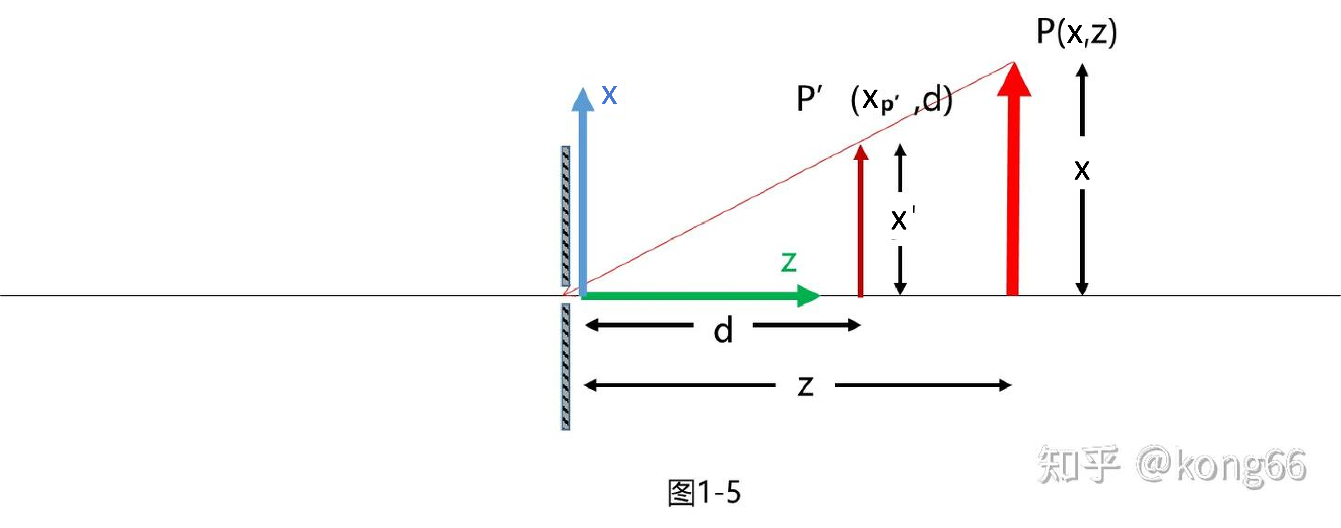
5.1.2.2 反转投影
其实这个$-d$是没有必要的, 反而增加计算的复杂度, 而且成像应该正过来, 因为这是计算机之中, 不是做小孔成像的实验. 它不需要严格遵守物理规律, 但是大小比例和真实情况是一样的. 此时的物体坐标点$P$和投影点$P'$的关系如上图所示, $P'$点的坐标为:$$x_{P'} = \frac{x}{z} \cdot d.$$
5.1.2.3 计算归一化投影坐标$x$
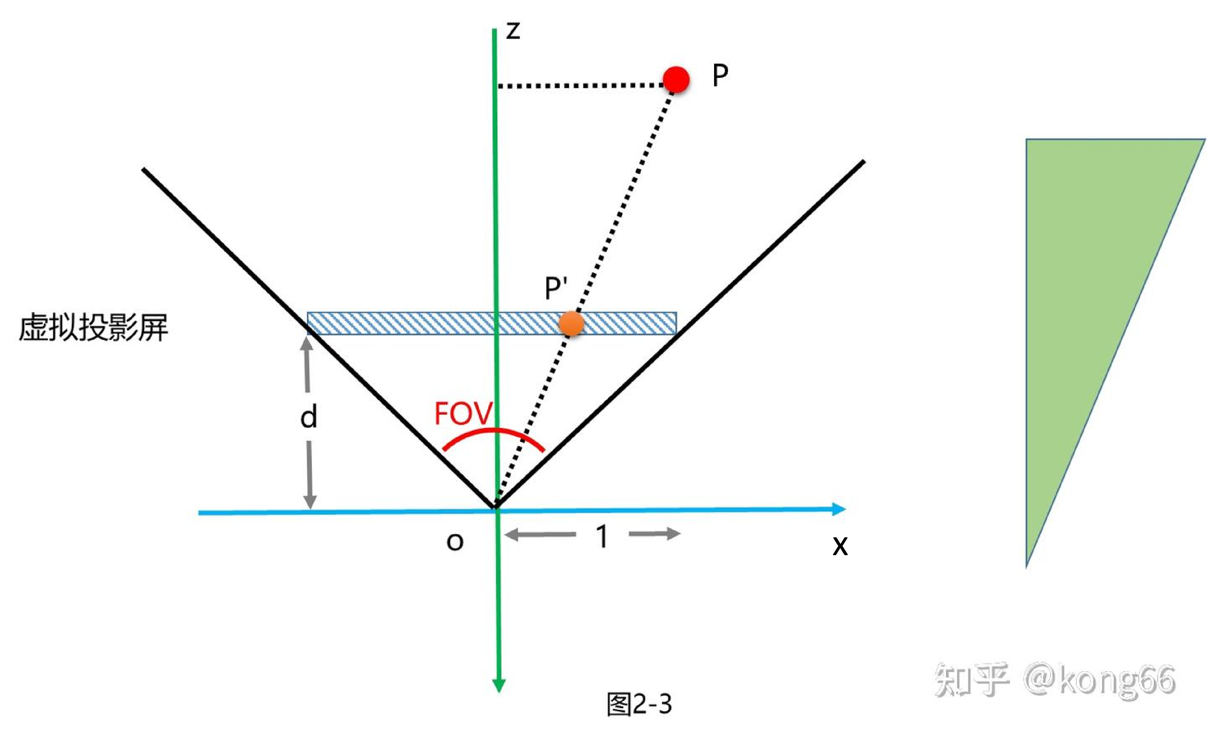
为了得到归一化的$x$坐标, 设置虚拟屏的宽度为2, 范围是$[-1, 1]$, 一半的尺寸就是1, 这是OpenGL的习惯, 如果是DirectX中, 这个范围是$[0, 1]$. 首先由FOV计算得到$d$, 再得到$x$坐标$$\frac{1}{d} = \tan\frac{FOV}{2}, \Rightarrow d = \frac{1}{\tan\frac{FOV}{2}}, \\ \frac{z_P}{z_{P'}} = \frac{x_P}{x_{P'}}, z_{P'} = -d = -\frac{1}{\tan\frac{FOV}{2}}, \\ \Rightarrow -\frac{z_P}{\frac{1}{\tan\frac{FOV}{2}}} = \frac{x_P}{x_{P'}}, \\ \Rightarrow x_{P'} = \frac{x_P \cdot \frac{1}{\tan\frac{FOV}{2}}}{z_P}, x_{P'} \in [-1, 1].$$
5.1.2.4 计算归一化投影坐标$y$
在垂直方向, 也遵循同样的投影规律, 而且无论计算$x$, 还是计算$y$, 都是同一块投影屏, 投影屏的坐标都是相同的, 都是$d$, 所以根据上式可以得到$$y_{P'} = -\frac{y_P \cdot d}{z_P} = -\frac{y_P \cdot \frac{1}{\tan\frac{FOV}{2}}}{z_P}, y_{P'} \in [-\frac{1}{A_{aspect}}, \frac{1}{A_{aspect}}].$$注意此时$y$坐标的取值范围不是想要的归一化的, 因为视锥体水平和垂直方向不一定是相等的, 是有宽高比的, 这个宽高比往往也是屏幕的宽高比, 所以当$w = 1$时, 为了画面不变形, 有$$\frac{w}{h} = A_{aspect}, h = \frac{w}{A_{aspect}} = \frac{1}{A_{aspect}}.$$但是, 为了得到归一化的$y$坐标,需要进行扩大操作, 即扩大$A_{aspect}$倍, 符合$[-1, 1]$的区间:$$y_{P'} = -\frac{y_P \cdot \frac{A_{aspect}}{\tan\frac{FOV}{2}}}{z_P}, y_{P'} \in [-\frac{A_{aspect}}{A_{aspect}}, \frac{A_{aspect}}{A_{aspect}}] = [-1, 1].$$
5.1.2.5 推导矩阵
通过上述式子可以得到最终的投影坐标, 如下式所示. 这个坐标不仅是归一化的, 而且已经除以了$\omega = z$, 已经是投影后的结果. 在下式中, $x$, $y$坐标的计算中可以找到$d$的部分, 但是$z$坐标中没有. \begin{equation} \left\{\begin{matrix}
x_{P'} = \frac{x_P \cdot \frac{1}{\tan\frac{FOV}{2}}}{z_P}, & x_{P'} \in [-1, 1], \\
y_{P'} = -\frac{y_P \cdot \frac{A_{aspect}}{\tan\frac{FOV}{2}}}{z_P}, & y_{P'} \in [-1, 1], \\
z_{P'} = -\frac{z_P \cdot (-\frac{f + n}{f - n}) - \frac{2nf}{f - n}}{z_P} & z_{P'} \in [-1, 1].
\end{matrix}\right. \label{final_projected_coordinates} \end{equation} 接下来将式$\ref{final_projected_coordinates}$还原为齐次坐标形式, 应为式$\ref{final_projected_coordinates_homogeneous_coordinate_form1}$, 执行齐次除法, 就是式$\ref{final_projected_coordinates}$. \begin{equation} \begin{pmatrix}
xd \\
yd \\
zd \\
\omega
\end{pmatrix} = \begin{pmatrix}
x_P \cdot \frac{1}{\tan\frac{FOV}{2}} \\
y_P \cdot \frac{A_{aspect}}{\tan\frac{FOV}{2}} \\
((z_P \cdot (-\frac{f + n}{f - n}) - \frac{2nf}{f - n}) \cdot \tan\frac{FOV}{2}) \cdot \frac{1}{\tan\frac{FOV}{2}} \\
-z_P
\end{pmatrix}, \\ d = \frac{1}{\tan\frac{FOV}{2}}, \omega = -z_P. \label{final_projected_coordinates_homogeneous_coordinate_form1} \end{equation} 如果将式$\ref{final_projected_coordinates}$还原为另一种齐次坐标形式, 应为式$\ref{final_projected_coordinates_homogeneous_coordinate_form2}$, 执行齐次除法, 就是式$\ref{final_projected_coordinates}$. \begin{equation} \begin{pmatrix}
x_{clip} \\
y_{clip} \\
z_{clip} \\
\omega
\end{pmatrix} = \begin{pmatrix}
x_P \cdot \frac{1}{\tan\frac{FOV}{2}} \\
y_P \cdot \frac{A_{aspect}}{\tan\frac{FOV}{2}} \\
(z_P \cdot (-\frac{f + n}{f - n}) - \frac{2nf}{f - n}) \\
-z_P
\end{pmatrix}, \\ d = \frac{1}{\tan\frac{FOV}{2}}, \omega = -z_P. \label{final_projected_coordinates_homogeneous_coordinate_form2} \end{equation}
想通过矩阵变换将一个观察空间的坐标$(x, y, z)$所对应的齐次坐标$(x, $$ y, z, 1)$, 转换到归一化的剪裁空间, 并且得到如式$\ref{final_projected_coordinates_homogeneous_coordinate_form2}$所示的形式, 这个形式执行一次齐次除法, 就能得到归一化的投影坐标:
$\\$ 投影矩阵 $\times$ 观察空间坐标 = 剪裁空间坐标, 如下式所示.$$M \begin{pmatrix}
x_P \\
y_P \\
z_P \\
1
\end{pmatrix} = \begin{pmatrix}
x_P \cdot \frac{1}{\tan\frac{FOV}{2}} \\
y_P \cdot \frac{A_{aspect}}{\tan\frac{FOV}{2}} \\
(z_P \cdot (-\frac{f + n}{f - n}) - \frac{2nf}{f - n} \\
-z_P
\end{pmatrix} = \begin{pmatrix}
x_{clip} \\
y_{clip} \\
z_{clip} \\
\omega
\end{pmatrix}, \\ \begin{pmatrix}
\frac{1}{\tan\frac{FOV}{2}} & 0 & 0 & 0 \\
0 & \frac{A_{aspect}}{\tan\frac{FOV}{2}} & 0 & 0 \\
0 & 0 & -\frac{f + n}{f - n} & - \frac{2nf}{f - n} \\
0 & 0 & -1 & 0
\end{pmatrix} \begin{pmatrix}
x_P \\
y_P \\
z_P \\
1
\end{pmatrix} = \begin{pmatrix}
x_P \cdot \frac{1}{\tan\frac{FOV}{2}} \\
y_P \cdot \frac{A_{aspect}}{\tan\frac{FOV}{2}} \\
(z_P \cdot (-\frac{f + n}{f - n}) - \frac{2nf}{f - n} \\
-z_P
\end{pmatrix}.$$最后得到的投影/ 剪裁矩阵如下式所示.$$M = \begin{pmatrix}
\frac{1}{\tan\frac{FOV}{2}} & 0 & 0 & 0 \\
0 & \frac{A_{aspect}}{\tan\frac{FOV}{2}} & 0 & 0 \\
0 & 0 & -\frac{f + n}{f - n} & - \frac{2nf}{f - n} \\
0 & 0 & -1 & 0
\end{pmatrix}.$$
5.2 矩阵转置处理
GPU上的矩阵表示与CPU上的表示不同. CPU上通常使用行矩阵, 而GPU上使用列矩阵. 因此, 在将矩阵传递到GPU之前, 需要进行转置处理, 确保数学运算的正确性.
6. 虚幻的ViewMatrix的变换流程
在Nanite渲染管线中, ViewMatrix的处理是关键第一步, 它决定了摄像机在世界空间中的位置和朝向. 课程中将ViewMatrix拆分为旋转和平移分量, 这为后续的Cluster选择提供了基础.
$\\$ ViewMatrix的数学结构是一个$4 \times 4$矩阵, 包含以下信息:
$\\$ $\cdot$ $3 \times 3$左上角: 摄像机的旋转矩阵(表示摄像机的方向);
$\\$ $\cdot$ 第四列前三行: 摄像机的位置向量的相反向量(表示摄像机在世界空间中的坐标各分量的相反数构成的坐标); 为了降低大世界Streaming下数值精度误差的影响, 虚幻引擎通常将World Space下的向量转换至Translated World Space下, 即将摄像机置于原点处, 故此时ViewMatrix的第四列前三行全为0;
$\\$ $\cdot$ 第四行第四列: 通常为1.0(齐次坐标).
$\\$ 拆分ViewMatrix的目的是为了单独处理摄像机的位置和朝向, 这在Cluster选择阶段非常重要. 必要情况下, 可以对摄像机参数进行压缩, 只保留必要的精度, 例如旋转和缩放参数通常不需要32位浮点数的精度.
7. 虚幻的自动化LOD的剔除逻辑
7.1 Clusters选择原理
Cluster是Nanite渲染管线的基本单位, 每个Cluster包含约128个三角形. Clusters选择的核心是判断Clusters在视口空间的投影是否可见. 这通过以下步骤实现:
$\\$ $\cdot$ 将Clusters的顶点从模型空间转换到视口空间;
$\\$ $\cdot$ 计算Clusters的屏幕空间投影范围;
$\\$ $\cdot$ 判断投影范围是否与视口相交.
$\\$ $\cdot$ 基于投影范围和误差阈值选择Mipmap Level.
$\\$ $\cdot$ 根据投影大小决定使用硬件或软件光栅化路径.
$\\$ Clusters选择必须在视口空间下进行, 因为这是摄像机观察的最终空间.
7.2 Clusters可见性判断
Clusters可见性判断是Nanite渲染管线的核心算法, 其核心代码如下所示:
//frustum volumen vs sphere,bvh node and cluster
//view space,world space
float2 GetProjectionScales(float4 inSphereWS){
	if(ProjectionMatrix[3][3]>=1.0f){//not ortho
		return float2(1.0f,1.0f);
	}
	//translated world
	//min z(0.1) * 0.1,max(0.9) z * 100.0
	float3 center=inSphereWS.xyz;
	float radius=inSphereWS.w;

	float distanceToSphereCenterSq=dot(center,center);
	float distanceToSphereCenter=sqrt(distanceToSphereCenterSq);

	float zVS=dot(Nanite_ViewForward.xyz,center);//center

	float xVSSq=distanceToSphereCenterSq-zVS*zVS;
	float xVS=sqrt(max(0.0f,xVSSq));

	float distanceToTangentPointSq=distanceToSphereCenterSq-radius*radius;
	float distanceToTangentPoint=sqrt(max(0.0f,distanceToTangentPointSq));

	float sinTheta=radius/distanceToSphereCenter;
	float cosTheta=distanceToTangentPoint/distanceToSphereCenter;

	float a=(-sinTheta*xVS+cosTheta*zVS)/distanceToSphereCenter;
	float b=(sinTheta*xVS+cosTheta*zVS)/distanceToSphereCenter;

	float minZ=max(10.0f,zVS-radius);
	float maxZ=max(10.0f,zVS+radius);

	if(zVS+radius>10.0f){
		return float2(minZ*a,maxZ*b);
	}
	return float2(0.0f,0.0f);
}
通过计算Clusters的包围球在视口范围内的投影缩放值, 可以快速确定Clusters是否可见.

上图可作为上述代码的示意图. 上述代码中函数GetProjectionScales的目的为了获取模型在视口空间中离摄像机最近点坐标的$z$分量值$minZ$, 该分量值会根据变量$a$的值进行一定程度上的缩放, 其中, 变量$a$的值是通过类似旋转变换的变换得到的; 而模型在视口空间中离摄像机最远点坐标的$z$分量值$maxZ$在虚幻中暂时未被使用.
7.2 Clusters剔除逻辑
Nanite的Clusters剔除逻辑: 第一阶段是对于BVH Nodes的初步筛选, 第二阶段是对于Clusters的精细剔除, 其伪代码如下所示.
// Compute Shader中Clusters剔除逻辑
[numthreads(1, 1, 1)]
void main(uint3 id : SV_GroupID) {
    // 获取BVH Node信息, 假设记录于id的x分量中
    uint BVHNodeIndex = id.x;
    BoundingSphere BVHNodeSphere = BVHNodeSpheres[BVHNodeIndex];

    // 计算BVHNode的LOD误差
    float BVHNodeLODError = CalculateBVHNodeLODErrors(BVHNodeSphere);

    // 第一阶段:对于BVH Nodes的初步筛选
    if (BVHNodeLODError > MaxLODError) {
        // 剔除,误差过大
        return;
    }

    // 获取Cluster信息, 假设记录于id的y分量中
    uint ClusterIndex = id.y;
    BoundingSphere ClusterSphere = ClusterSpheres[ClusterIndex];

    // 计算Cluster的LOD误差
    float ClusterLODError = CalculateClusterLODErrors(ClusterSphere);

    // 第二阶段:对于Clusters的精细剔除
    if (!CheckVisibility(ClusterSphere, ClusterLODError)) {
        // 剔除,不可见
        return;
    }

    // 标记为可见
    VisibleClusterIndices[id.x] = ClusterIndex;
}
$\cdot$ 初步筛选阶段基于LOD误差判断, 剔除那些即使在最佳Mipmap Level下也无法满足视觉质量要求的BVH Nodes, 即剔除不满足LOD Error上限的BVH Nodes, 其核心代码如下所示.
bool ShouldVisitChild(FHierarchyNodeSlice inHierarchyNodeSlice){
	float3 boundingSphere=inHierarchyNodeSlice.LODBounds.xyz;
	float4 boundingSpherePositionWS=mul(ModelMatrix,float4(boundingSphere,1.0f));
	boundingSpherePositionWS=float4(boundingSpherePositionWS.xyz-Nanite_ViewOrigin.xyz,1.0f);
	//QEM : Quadric Error Metrics,METIS
	float2 projectionScales=GetProjectionScales(float4(boundingSpherePositionWS.xyz,inHierarchyNodeSlice.LODBounds.w));
	float lodScale=Nanite_ViewOrigin.w;
	float threshold=lodScale*inHierarchyNodeSlice.MaxParentLODError;
	if(projectionScales.x<=threshold){
		//projectionScales.y>minLODError
		return true;
	}
	return false;
}
$\cdot$ 精细剔除阶段基于Clusters的包围球在视口范围内的投影缩放值判断, 进一步剔除那些不满足LOD Error下限的Clusters, 其核心代码如下所示.
//View Direction (World Space),depth
//Translated World
//View Matrix : RotationScale + Translate + ViewForward
//Projection Matrix,fov : y => x : x,y,z
//0~1024 : cluster 0~n
//4096~2048 : cluster n ~ 0
[numthreads(1,1,1)]//1 -> wave : 32
void MainCS(){
	uint clusterCount=WorkArg.Load2(0).y;
	uint visibleClusterCount=0;
	for(uint i=0;i < clusterCount;i++){
		uint2 packedCluster=MainAndPostNodeAndClusterBatches.Load2(i*8u);
		uint pageIndex=packedCluster.x;
		uint clusterIndex=packedCluster.y;//MipLevel,LODBounds,LODError,EdgeLength => SW,HW,Visible(false)
		ClusterInfo clusterInfo=GetClusterinfo(pageIndex,clusterIndex);
		float3 boundingSphere=clusterInfo.LODBounds.xyz;
		float4 boundingSpherePositionWS=mul(ModelMatrix,float4(boundingSphere,1.0f));
		boundingSpherePositionWS=float4(boundingSpherePositionWS.xyz-Nanite_ViewOrigin.xyz,1.0f);
		//QEM : Quadric Error Metrics,METIS
		float2 projectionScales=GetProjectionScales(float4(boundingSpherePositionWS.xyz,clusterInfo.LODBounds.w));
		float lodScale=Nanite_ViewOrigin.w;
		float lodScaleHW=Nanite_ViewForward.w;
		if(projectionScales.x > clusterInfo.LODError*lodScale){
			if(projectionScales.x < abs(clusterInfo.EdgeLength)*lodScaleHW){
				//hw
			}else{
				//sw
			}
			OutVisibleClustersSWHW.Store2(visibleClusterCount*8u,packedCluster);
			visibleClusterCount++;
		}
	}
	WorkArg.Store(4,visibleClusterCount);
}